Generate ficus benjamina leaf shapes with bezier curves • ggbenjamini

Generate benjamini leaves with bezier curves

The goal of this package is to generate shapes in the form of ficus benjamina leaves (weeping fig) with bezier curves. It is heavily inspired by the awesome flametree package.

Installation

You can install the newest version of ggbenjamini from github with:

# install.packages("remotes")
# (if not installed yet)

remotes::install_github("urswilke/ggbenjamini")

Usage

First load some libraries:

library(ggbenjamini)
library(purrr)
library(dplyr)
library(tidyr)
library(stringr)
library(ggplot2)
library(ggforce)
set.seed(123)

Illustration of the generated data

The package generates bezier curves that imitate the shape of the leaves of a ficus benjamini. The main function is benjamini_leaf():

df <- benjamini_leaf()

Show generated dataframe df of benjamini leaf bezier curve parameters

knitr::kable(df)

element	i_part	x	y	param_type
stalk	0	10.00000	40.00000	bezier start point
stalk	0	10.04566	40.94991	bezier control point 1
stalk	0	19.97942	39.35523	bezier control point 2
stalk	0	20.00000	40.00000	bezier end point
half 2	1	20.00000	40.00000	bezier start point
half 2	1	22.00000	36.00000	bezier control point 1
half 2	1	29.00000	35.17208	bezier control point 2
half 2	1	34.00000	35.00000	bezier end point
half 2	2	34.00000	35.00000	bezier start point
half 2	2	39.00000	34.82792	bezier control point 1
half 2	2	43.00000	37.33259	bezier control point 2
half 2	2	45.00000	38.78709	bezier end point
half 2	3	45.00000	38.78709	bezier start point
half 2	3	47.00000	40.24159	bezier control point 1
half 2	3	50.97942	39.35523	bezier control point 2
half 2	3	51.00000	40.00000	bezier end point
half 2	4	51.00000	40.00000	bezier start point
half 2	4	38.00000	40.31141	bezier control point 1
half 2	4	33.00000	39.58294	bezier control point 2
half 2	4	20.00000	40.00000	bezier end point
half 1	1	20.00000	40.00000	bezier start point
half 1	1	22.00000	44.00000	bezier control point 1
half 1	1	29.00000	44.82792	bezier control point 2
half 1	1	34.00000	45.00000	bezier end point
half 1	2	34.00000	45.00000	bezier start point
half 1	2	39.00000	45.17208	bezier control point 1
half 1	2	43.00000	42.66741	bezier control point 2
half 1	2	45.00000	41.21291	bezier end point
half 1	3	45.00000	41.21291	bezier start point
half 1	3	47.00000	39.75841	bezier control point 1
half 1	3	50.97942	40.64477	bezier control point 2
half 1	3	51.00000	40.00000	bezier end point
half 1	4	51.00000	40.00000	bezier start point
half 1	4	38.00000	40.31141	bezier control point 1
half 1	4	33.00000	39.58294	bezier control point 2
half 1	4	20.00000	40.00000	bezier end point

It results in a dataframe of multiple bezier curves representing the shape of a leaf. The first column element indicates which part of the leaf the bezier describes, and can take the values “stalk”, “half 2” and “half 1”. i_part denotes the id of the bezier curve, and x & y its point coordinates. The column param_type denotes the type of the point in the bezier curve.

The meaning is best illustrated with a plot:

Show code to generate plot

# rearrange data to display segments:
segments <- df %>% 
  select(-param_type) %>% 
  group_by(element, i_part) %>% 
  mutate(j = c(1, 2, 1, 2)) %>%
  ungroup() %>% 
  pivot_wider(
    names_from = j,
    values_from = c(x, y),
    values_fn = list
  ) %>% 
  unnest(c(x_1, x_2, y_1, y_2))

p <- ggplot(df, aes(x = x, y = y)) + 
  geom_point(color = "red") +
  geom_point(
    data = df %>% 
      group_by(element, i_part) %>% 
      slice(c(1, 4)),
    color = "blue", 
    size = 2
  ) +
  geom_point(
    data = df %>% slice(1), 
    color = "black", 
    size = 3
  ) +
  geom_bezier(
    aes(
      group = interaction(element, i_part), 
      color = factor(i_part)
    )) +
  geom_segment(
    data = segments, 
    aes(
      x = x_1, 
      xend = x_2, 
      y = y_1, 
      yend = y_2
    ), 
    linetype = "dotted", 
    color = "red"
  ) +
  coord_equal() +
  theme_minimal()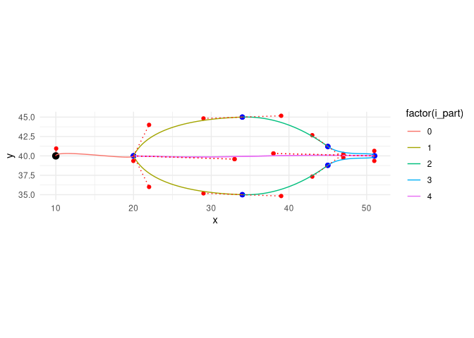

The black point represents the leaf origin. Together with the blue points they denote the start/end points of the bezier curves, and the red dots the positions of their control points. The leaf is cut in two halves (element == "half 1" OR "half 2") by the lines where i_part == 4 (which represents the midvein of the leaf). The exact dimensions of these coordinates are generated by random numbers in certain ranges (see the definition of the argument leaf_params in benjamini_leaf()).

Illustration of the randomness

In order to show the variations of the benjamini_leaf() (if parameters are not explicitly specified), let’s only pass the position of the leaf origins and let the function randomly generate the rest of the shapes:

dfb <- expand_grid(
    x = seq(0, 200, 50),
    y = seq(25, 125, 25)
) %>%
  transpose() %>%
  map_dfr(
    ~benjamini_leaf(gen_leaf_parameters(
      x0 = .x$x, 
      y0 = .x$y
    )), 
    .id = "i_leaf"
  ) %>%
  unite(i, i_leaf, i_part, element, remove = FALSE)

ggplot(dfb) +
  geom_bezier(aes(x = x, y = y, group = i)) +
  coord_equal() +
  theme_minimal()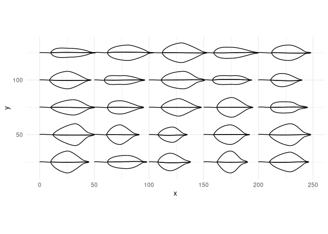

Branches

You can also generate branches of leaves with the command benjamini_branch() (see the vignettes vignette("create_benjamini_polygons") and vignette("create_benjamini_tree") for examples):

df_branch <- benjamini_branch() %>%
  # we add a unique identifier `b` for all beziers:
  unite(b, i_leaf, element, i_part, remove = FALSE) 
df_branch
#> # A tibble: 436 × 8
#>    b          i_leaf element i_part     x     y type        param_type    
#>    <chr>       <dbl> <chr>    <dbl> <dbl> <dbl> <chr>       <chr>         
#>  1 0_branch_1      0 branch       1  70    280  branch      bezier start …
#>  2 0_branch_1      0 branch       1  84    245  branch      bezier contro…
#>  3 0_branch_1      0 branch       1 126    217  branch      bezier contro…
#>  4 0_branch_1      0 branch       1 168    217  branch      bezier end po…
#>  5 1_stalk_0       1 stalk        0  75.7  269. leaf_bezier bezier start …
#>  6 1_stalk_0       1 stalk        0  76.2  268. leaf_bezier bezier contro…
#>  7 1_stalk_0       1 stalk        0  73.8  264  leaf_bezier bezier contro…
#>  8 1_stalk_0       1 stalk        0  74.0  264. leaf_bezier bezier end po…
#>  9 1_half 2_1      1 half 2       1  74.0  264. leaf_bezier bezier start …
#> 10 1_half 2_1      1 half 2       1  71.4  264. leaf_bezier bezier contro…
#> # ℹ 426 more rows

As the following plot also shows, benjamini_branch() adds another column i_leaf specifying the index of the leaf on the branch.

df_branch %>%
  ggplot() +
  geom_bezier(aes(x = x, y = y, group = b, color = i_leaf)) +
  coord_equal()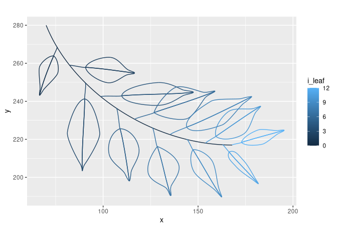

Polygons

If you want to fill the leaves with color, you can use bezier_to_polygon() to approximate the bezier curves leaf parts with polygons:

df_polygons <- df_branch %>% 
  filter(str_detect(element, "^half [12]$")) %>%
  unite(idx, i_leaf, element, remove = FALSE) %>%
  bezier_to_polygon(idx, i_leaf, element, i_part, n = 100)
ggplot(
  data = df_polygons,
  aes(x = x, y = y, group = idx, fill = i_leaf)
) +
  geom_polygon(show.legend = FALSE, color = "black") +
  scale_fill_gradientn(colours = c("darkgreen", "green")) +
  theme_void()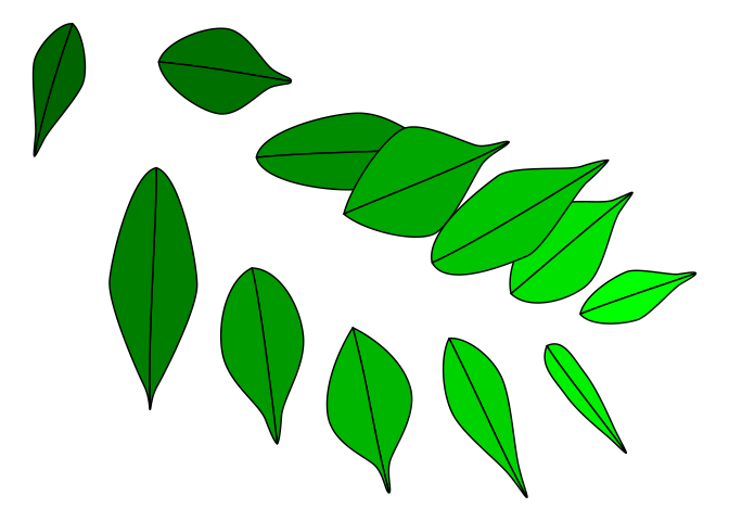

If you want to know more have a look in vignette("create_benjamini_polygons") .

svg

You can also transform the leaf data to svgs. Have a look in vignette("create_benjamini_svg") for an example to generate svg images.

R packages used

This package stands on the shoulders of giants. It was only possible thanks to the following libraries:

base (R Core Team 2021a)
tidyverse (Wickham et al. 2019)
ggforce (Pedersen 2021)
grid (R Core Team 2021b)
prismatic (Hvitfeldt 2021)
flametree (Navarro 2021)
rsvg (Ooms 2021b)
minisvg (FC 2021)
ambient (Pedersen and Peck 2020)
covr (Hester 2020)
stats (R Core Team 2021c)
magick (Ooms 2021a)

References

FC, Mike. 2021. Minisvg: SVG Document Builder.

Hester, Jim. 2020. Covr: Test Coverage for Packages. https://CRAN.R-project.org/package=covr.

Hvitfeldt, Emil. 2021. Prismatic: Color Manipulation Tools. https://CRAN.R-project.org/package=prismatic.

Navarro, Danielle. 2021. Flametree: Generate Random Tree-Like Images. https://CRAN.R-project.org/package=flametree.

Ooms, Jeroen. 2021a. Magick: Advanced Graphics and Image-Processing in r. https://CRAN.R-project.org/package=magick.

———. 2021b. Rsvg: Render SVG Images into PDF, PNG, PostScript, or Bitmap Arrays. https://CRAN.R-project.org/package=rsvg.

Pedersen, Thomas Lin. 2021. Ggforce: Accelerating ’Ggplot2’. https://CRAN.R-project.org/package=ggforce.

Pedersen, Thomas Lin, and Jordan Peck. 2020. Ambient: A Generator of Multidimensional Noise. https://CRAN.R-project.org/package=ambient.

R Core Team. 2021a. R: A Language and Environment for Statistical Computing. Vienna, Austria: R Foundation for Statistical Computing. https://www.R-project.org/.

———. 2021b. R: A Language and Environment for Statistical Computing. Vienna, Austria: R Foundation for Statistical Computing. https://www.R-project.org/.

———. 2021c. R: A Language and Environment for Statistical Computing. Vienna, Austria: R Foundation for Statistical Computing. https://www.R-project.org/.

Wickham, Hadley, Mara Averick, Jennifer Bryan, Winston Chang, Lucy D’Agostino McGowan, Romain François, Garrett Grolemund, et al. 2019. “Welcome to the tidyverse.” Journal of Open Source Software 4 (43): 1686. https://doi.org/10.21105/joss.01686.